最小二乗法 ¶

本稿では SciPy を用いて最小二乗法問題の扱いについて記す。これも NumPy だけでなんとかなる問題だが、やってみよう。

関数 `scipy.linalg.lstsq`¶

関数 scipy.linalg.lstsq を呼び出すことで、測定データなり抽出データなりの最小二乗法による回帰曲線（直線）を求められる。実用の都合上、測定値は二次元の平面に直線的に（一次関数の形で）分布するという条件での方法を記す。

コード的な手順は次のとおりとなる。

測定データを x, y 座標ごとに array_like オブジェクトの形で用意する。本説明ではそれぞれ xd, yd とする。

行列 A を次のように設定する。

A = [[xd[0], 1], [xd[1], 1], ..., [xd[-1], 1]]

ベクトル B を yd とする。
lstsq(A, B) を呼び出す。戻り値の tuple の最初の要素を X とする。これも tuple である。
X の最初の要素と次の要素が回帰直線の傾きと切片である。本説明ではそれぞれ a, b とする。

コード例を示す。

#!/usr/bin/env python
"""least_squares.py: Demonstrate least-squares fitting method of SciPy.

References:
  * http://sagemath.wikispaces.com/numpy.linalg.lstsq
"""
from scipy.linalg import lstsq
import numpy as np
import matplotlib.pyplot as plt

# pylint: disable=invalid-name

# Sampling data set.
xd = np.array([72, 67, 65, 55, 25, 36, 56, 34,
               18, 71, 67, 48, 72, 51, 53])
yd = np.array([202, 186, 187, 180, 156, 169, 174,
               172, 153, 199, 193, 174, 198, 183, 178])

# Solve the linear least squares problem.
A = np.c_[xd[:, np.newaxis], np.ones(xd.shape[0])]
B = yd
X, residues, rank, s = lstsq(A, B)

# Show the regression curve (line).
a = X[0]
b = X[1]
print(f"Line: y = {a:.3f}x {b:+.3f}")

# Plot both the sampling data and the regression curve.
# pylint: disable=invalid-slice-index
plt.figure()
xs = np.r_[min(xd):max(xd):15j]
ys = a * xs + b

plt.plot(xs, ys, color='deeppink', label='regression curve')
plt.scatter(xd, yd, color='pink', marker='s', label='data set')
plt.legend()
plt.show()

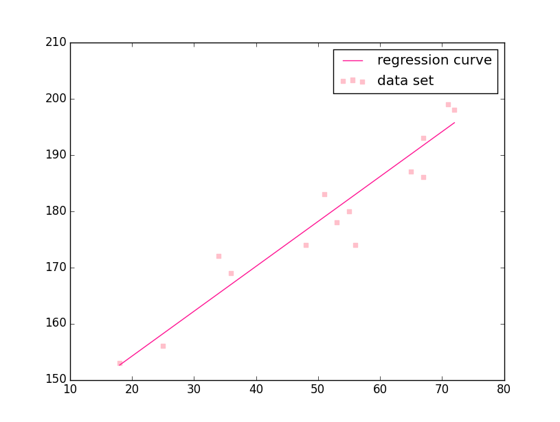
私の環境での実行結果は次のとおり。

Line: y = 0.798x +138.253

回帰直線が得られたので、測定データと同時にグラフを描くとこのようになる。

最小二乗法¶

関数 scipy.linalg.lstsq¶

最小二乗法 ¶

関数 `scipy.linalg.lstsq`¶