常微分方程式 ¶

本稿では SciPy を用いて簡単な微分方程式の数値計算を行う。どうも偏微分方程式は現時点では未実装らしいので、常微分方程式だけを解くことにする。

Note

SymPy の利用も検討したい。

関数 `scipy.integrate.odeint`¶

関数 scipy.integrate.odeint を利用することで、常微分方程式を数値的に解くことができる場合がある。

コード的な手順は次のとおりとなる。これはもっとも単純な使い方に過ぎない。

後述のコード例中に見られるような関数 deriv を定義する。
- 第一引数が微分方程式中の未知関数。本説明では y とする。
- 第二引数が関数のパラメーター。本説明では t とする。
- 戻り値がパラメーター t における [一次微分, 二次微分, ...] を意味する。
未知関数の定義域に亘るパラメーター列を用意する。後述コード例の time が相当する。
微分方程式の初期値（初期条件）を数値で与える。後述コード例の yinit が相当する。
関数 scipy.integrate.odeint に三者を引数にして呼び出す。
- 戻り値が time 各パラメーターに対応する未知関数 y の各値である。

コード例を示す。定数係数 2 階線形微分方程式を解くものだ。

#!/usr/bin/env python
"""odeint.py: Demonstrate solving an ordinary differential equation by using
odeint.

References:
  * Solving Ordinary Differential Equations (ODEs) using Python
"""
from scipy.integrate import odeint
import numpy as np
import matplotlib.pyplot as plt

# pylint: disable=invalid-name

# Solve y''(t) + a y'(t) + b y(t) == 0.

# pylint: disable=unused-argument
def deriv(y, t):
    """Return derivatives of the array y."""
    a = 3.0
    b = 2.0
    # y[0] : y'
    # y[1] : y''
    return np.array([
        y[1], # (y[0])'
        -(a * y[0] + b * y[1]) # (y[1])'
        ])

time = np.linspace(0.0, 10.0, 1000)
yinit = np.array([0.0005, 0.2]) # initial values
y = odeint(deriv, yinit, time)

plt.figure()
# y[:,0] is the first column of y
plt.plot(time, y[:, 0], color='deeppink')
plt.xlabel("t")
plt.ylabel("y")
plt.show()

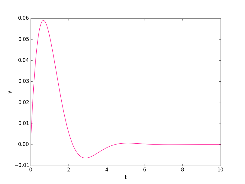
私の環境での実行結果は次のとおり。いつものような print ではプログラムの実行内容がさすがに理解不能なので、本稿はプロットによるグラフ描画の出力を示す。微分方程式 \({y'' +3y' + 2y = 0}\) は \({y = C_1 e^{-x} + C_2 \mathrm{e}^{-2x}}\) が一般解であり、図の曲線はそのように見えるだろう。

Note

SymPy ならばこのようになる：

In [1]: dsolve(f(x).diff(x, 2) + 3 * f(x).diff(x) + 2 * f(x))
Out[1]: Eq(f(x), (C1 + C2*exp(-x))*exp(-x))

常微分方程式¶

関数 scipy.integrate.odeint¶

常微分方程式 ¶

関数 `scipy.integrate.odeint`¶